StatsPy Users Guide ¶

Contents

StatsPy Users Guide

Introduction ¶

StatsPy is a python based statistical package aimed to help users to build conveniently relatively complex probability functions which can be used later to fit to data, perform statistical tests or extract confidence intervals. StatsPy is originally inspired from the RooFit/RooStats packages used in High Energy Physics within the CERN ROOT analysis framework. The main two motivations for creating a new tool were to build a framework directly from python and thus oriented toward the “pythonic” scripting style, and to create a package built on top of the widely used NumPy/SciPy scientific stack.

The package development is yet at its beginning and currently focused on the main elements to build conveniently a probability function.

StatsPy Quick Start ¶

Conventions ¶

As many packages, StatsPy relies heavily on acronyms. The main ones are used to define the 3 basic classes used in StatsPy.

PF = Probability Function, a generic name, following Kendall’s Advanced Theory of Statistics, referring both to Probability Density Functions (PDF/pdf) in the case of continuous random variables and to Probability Mass Functions (PMF/pmf) for discrete random variables.
RV = Random Variable, which is self explanatory.
Param = Parameters denote quantities that appear specifically in the specification of the probability function. In the present package, any function of parameters will be also named a parameter, and such quantities are named DERIVED in opposition to RAW parameters.

Probability Functions ¶

Declaration and evaluation ¶

Probability functions are declared via the base class statspy.core.PF

Example 1, declare and call a normal distribution:

>>> import statspy as sp
>>> mypdf = sp.PF("pdf_norm=norm(x;mu=20,sigma=5)")

In this case the whole PF is defined via the string argument

pdf_norm, the name of the PF is defined on the left-hand side of the assignment statement sign (“=”). Giving a name to a PF is optional but recommended. The name can be retrieved via:
```
>>> mypdf.name
pdf_norm
```
norm is a keyword referring to the scipy.stats.norm function which is used to compute the actual value of the PF. Any pdf or pmf defined in the scipy.stats module can be used as a keyword. The statistical function should be followed by parenthesis.
Within the parenthesis, the first part should be used to define the name of the random variable(s), x, in the case above.
The second part of the parenthesis defines the list of shape parameters used to define a normal distribution, i.e. its mean and its rms. Their order should follow the one used by the scipy.stats.norm function. The shape parameters are separated from the random variables via the ”;” or “|” characters. If a shape parameter is new, it is automatically declared and registered within some internal dictionary. If a shape parameter has already been declared, the PF is linked toward it. It is possible to retrieve a Parameter via the function get_obj(name):
```
>>> mu = sp.get_obj("mu")
>>> mu.value
20
```

Alternatively keyword arguments can be used to set various PF members:

>>> poisson_pmf = sp.PF("poisson(n|lbda)",name="pmf_poisson",lbda=10)

To evaluate the probability function in x, the special method __call__ is used. x can be either a float or an array:

>>> mypdf(25)
0.048394144903828672
>>> import numpy as np
>>> import matplotlib.pyplot as plt
>>> x = np.linspace(0,40,400)
>>> plt.plot(x,mypdf(x),'r-')
>>> plt.show()

Since available in scipy.stats, the cumulative distribution function (PF.cdf), the survival function (PF.sf = 1 - PF.cdf), and the logarithm of the probability function (PF.logpf) can be evaluated via:

>>> plt.plot(x,mypdf.cdf(x))
>>> plt.plot(x,mypdf.sf(x))
>>> plt.show()
>>> plt.plot(x,-mypdf.logpf(x))
>>> plt.show()

Finally, as in scipy.stats, it is possible to generate random variates using the function (PF.rvs):

>>> mypdf.rvs(size=10)

Operations with PFs ¶

The methods seen in the first section do not really bring value with respect to scipy.stats and are heavily relying on them. The real gain of StatsPy is the possibility to conveniently build new PFs from existing PFs via different operations:

addition of different PFs, for example if there is a random signal on top of a random background.
Example 2: a normally distributed signal on top of an exponentially falling background can be easily modelled with the following syntax:
>>> import numpy as np >>> import statspy as sp >>> import matplotlib.pyplot as plt >>> pdf_true_sig = sp.PF("pdf_true_sig=norm(x;mu_true=125,sigma_true=10)") >>> pdf_true_bkg = sp.PF("pdf_true_bkg=expon(x;offset_true=50,lambda_true=20)") >>> pdf_true = 0.95 * pdf_true_bkg + 0.05 * pdf_true_sig >>> x = np.linspace(50,200,150) >>> plt.plot(x,pdf_true(x)) >>> plt.plot(x,pdf_true_bkg(x)) >>> plt.plot(x,pdf_true_sig(x)) >>> plt.show()
When adding the two pdf pdf_true_sig and pdf_true, their normalization coefficients become nested. If c_sig and c_bkg are the normalization coefficients of pdf_true_sig and pdf_true respectively, then c_bkg is redefined as a DERIVED parameter c_bkg = 1 - c_sig. Similarly, if n PFs are added with c_i coefficients respectively, then c_1 is defined as 1 - sum(i=2,i=n) c_i.

multiplication of PFs as when combining PFs applying to different random variables.

Example 3: product of two Poisson distributions:

>>> import numpy as np
>>> import statspy as sp
>>> import matplotlib.pyplot as plt
>>> pmf_on  = sp.PF('pmf_on=poisson(n_on;mu_on=1)')
>>> pmf_off = sp.PF('pmf_off=poisson(n_off;mu_off=5)')
>>> likelihood = pmf_on * pmf_off
>>> x = y = np.arange(0, 20)
>>> X, Y = np.meshgrid(x, y)
>>> from matplotlib import ticker
>>> plt.contourf(X, Y, likelihood(X,Y), locator=ticker.LogLocator())
>>> plt.show()

Other operations like convolutions will be presented in the section dedicated to Working with Random Variables.

An interlude about parameters ¶

Very often, in practical statistical inference problems, one wants to estimate parameters which are not directly related to the parameters defining the pdf/pmf. The core.Param class is designed such as it is relatively easy to define DERIVED parameters from other parameters. The DERIVED parameters can then be used to construct the different pdf/pmf.

Example 3 (Con’t): As an example, in the on/off problem, one is modelling a counting device like a CCD camera behind a telescope. When the telescope is pointing toward a source n_on events are counted, while n_off photons are found with the telescope pointing at a source-free direction. n_on is sensitive to the source signal rate s which one tries to evaluate and to other sources leading to a background rate b. n_off is a subsidiary measurement sensitive to b only. In practice, one will model this problem with StatsPy via:

>>> import statspy as sp
>>> mu = sp.Param("mu = 0.", poi=True) # Signal strength
>>> s = sp.Param("s = 3.", const=True) # Expected number of signal evts
>>> b = sp.Param("b = 1.") # Expected number of bkg evts in signal region
>>> tau = sp.Param("tau = 5.", const=True)
>>> mu_on  = mu * s + b # Total events expectation in the signal region
>>> mu_off = tau*b      # Total events expectation in the control region

Then the pmf and the likelihood can be defined like:

>>> pmf_on  = sp.PF('pmf_on=poisson(n_on;mu_on)')
>>> pmf_off = sp.PF('pmf_off=poisson(n_off;mu_off)')
>>> likelihood = pmf_on * pmf_off

In particular from the example above

mu_on and mu_off are what is called DERIVED parameters meaning they are constructed from other parameters. When the value of mu or b is changed, it gets automatically propagated to mu_on and mu_off and the relevant pmf.
A parameter like s or tau can be defined as const=True. It means that during fits, the parameter will be fixed to its value.
For hypothesis tests, it is necessary to distinguish between parameters of interest (poi) and nuisance parameters. It is done by specifying poi=True as for mu the signal strength in the on/off example.

Perform a fit to data ¶

To perform a fit to data, two methods are provided in the PF class: the least square method leastsq_fit and the maximum likelihood method maxlikelihood_fit.

Example 2 (Con’t): considering again the example of a normally distributed signal on top of an exponentially falling background, a least-square fit would be done like:

# Define the background and signal PFs
pdf_fit_bkg = sp.PF("pdf_fit_bkg=expon(x;offset=50,lambda=10)")
pdf_fit_sig = sp.PF("pdf_fit_sig=norm(x;mu=120,sigma=20)")
pdf_fit = pdf_fit_bkg + pdf_fit_sig
pdf_fit_sig.norm.label = 'frac(sig)'
# Least square fit to the data (whole data range)

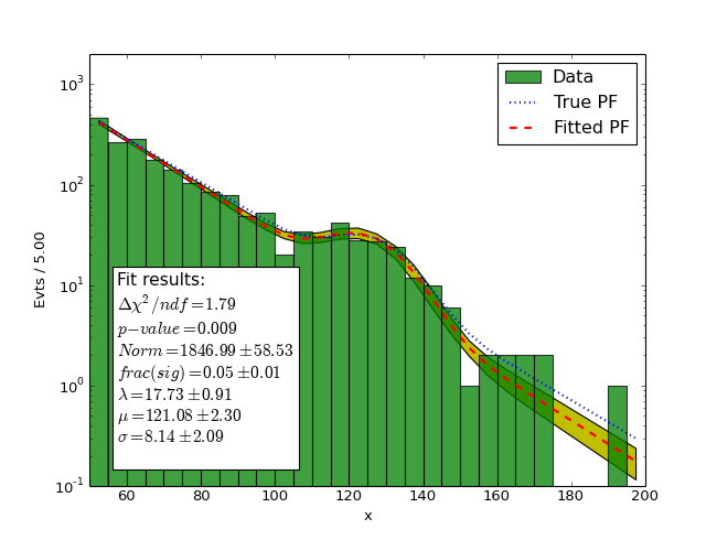
(Source code, png)

Working with Random Variables ¶

It is sometimes easier to think a problem in term of random variable than in term of probability functions. We also might want to know the probability function of a random variable given its formula as a function of other random variables. The class statspy.core.RV is designed to solve some of these problems (rescaling, additions, multplicitations) numerically.

Random variables are declared with a similar syntax to PF:

>>> import statspy as sp
>>> X = sp.RV("norm(x|mu=10,sigma=2)")

To access the PF associated to a Random Variable and its methods, the self.pf class member should be used:

>>> X.pf(12)
0.12098536225957168
>>> X.pf.cdf(12)
0.84134474606854293

and radom variates can be generated directly via the __call__ special method:

>>> X(size=10)

But the main usage of this class it to determine the PF of derived random variables as illustrated by the code snippets and figure below.

X = sp.RV("norm(x;mux=15,sigmax=3)")
Y = sp.RV("norm(y;muy=10,sigmay=4)")
Z1 = X + Y
Z2 = X - Y
mux = sp.get_obj('mux')
sigmax = sp.get_obj('sigmax')
Z5 = (X - mux) / sigmax

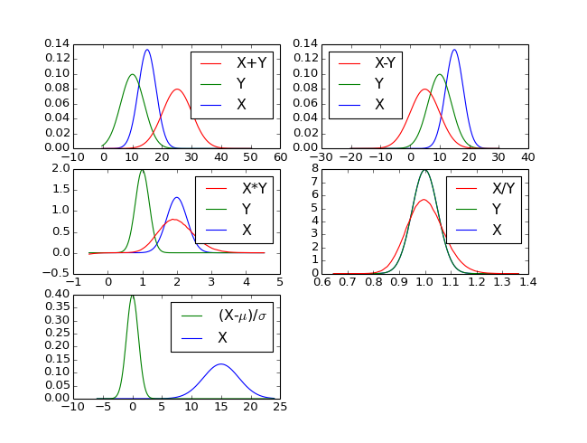
(Source code, png)

Statistical inference with StatsPy ¶

Parameters estimation ¶

The free parameters (i.e. parameters for which Param.const == False) of a probability function can be fitted to data via two widely used methods.

The method of least squares which requires as minimial inputs the x- and y- values of a set of data has already been illustrated in the Perform a fit to data section. After running a least square fit, the free parameters of the fit have their value updated but also their uncertainty unc. Uncertainties and correlations between free parameters are computed using some approximation of the Hessian matrix.

The maximum likelihood estimation only requires as input random variates:

>>> import statspy as sp
>>> pdf_true = sp.PF("pdf_true=norm(x|mu_true=20.,sigma_true=5.)")
>>> data = pdf_true.rvs(size=20)
>>> pdf_fit = sp.PF("pdf_fit=norm(x|mu_fit=1.,sigma_fit=1.)")
>>> pdf_fit.maxlikelihood_fit(data)
([mu_fit = 19.5111374418, sigma_fit = 5.12291410326], 41.053294585533187)

Intervals estimation ¶

Interval estimation allows one to not only quote a point estimate of a parameter but an interval of possible values. They are named confidence intervals in a frequentist approach and credible intervals with a Bayesian method. The aim of the module statspy.interval is provide functions to conveniently compute both type of intervals.

Note

currently only the PLLR method (popular in HEP) is provided. Aim is to add another method (Neyman construction) and a Bayesian method

The profile (log-)likelihood ratio (PLLR) method is an approximate frequentist approach relying on the profile likelihood ratio test statistics and the Wilks’ theorem to build confidence intervals. Its main advantage with respect to other frequentist methods like the Neyman construction is its speed and the possibility to apply it also in problems with a large number of (nuisance) parameters. To get an approximate confidence interval on a parameter θ_i , the algorithm consists in:
- Get the maximum likelihood estimate θ̂_i as central value
- Define a profile log-likehood ratio function q(θ_i) as
  
  Λ(θ_i) = (L(x|θ_i, θ̂̂_s))/(L(x|θ̂_i, θ̂_s))
  
  q(θ_i) = − 2log(Λ(θ_i))
  
  where L(x|θ_i, θ̂̂_s) and L(x|θ̂_i, θ̂_s) are the conditional and unconditional maximum of the likelihood function respectively.
- Search for values of q(θ_i) equaling quantile defined as:
```
quantile = scipy.stats.chi2.ppf(cl, ndf)
```
  where cl is the confidence level and ndf the number of degrees of freedom. This formula relies on the fact that the profile likelihood ratio is asymptotically distributed by a chi2 function (Wilks’ theorem). In practical cases, it is therefore an approximation which can be verified with a toy MC technique.

Hypothesis tests ¶

As for interval estimation, the module statspy.hypotest provides methods to perform hypothesis tests.

Quoting “Kendall’s Advanced Theory of Statistics”, the likelihood ratio method has played a role in the theory of tests analogous to that of the maximum likelihood method in the theory of estimation. Generally, one wish to test the null hypothesis

H₀:θ_r = θ_r0

against the alternative hypothesis

H₁:θ_r ≠ θ_r0

taking into accound a number of nuisance parameters θ_s . As for the likelihood ratio method used for interval estimation, one defines the log-likehood ratio test statistics as

Λ(θ_r0) = (L(x|θ_r0, θ̂̂_s))/(L(x|θ̂_r, θ̂_s))

q(θ_r0) = − 2log(Λ(θ_r0))

with L(x|θ_r0, θ̂̂_s) and L(x|θ̂_r, θ̂_s) the conditional and unconditional maximum of the likelihood function respectively. Asymptotically q(θ_r0) is distributed as a chi2 function from which p-value or Z-value can be computed. If the p-value is lower than a predefined type I error rate, then the null hypothesis is rejected.

Example 3 (Con’t): considering again the on/off problem, to perform a likelihood ratio test on the background only hypothesis (mu=0), one would do:
```
>>> data = (4, 5) # n_on, n_off
>>> import statspy.hypotest
>>> result = statspy.hypotest.pllr(likelihood, data)
>>> print 'p-value',result.pvalue,'Z-score',result.Zvalue
```